Introduction to Analysis of Variance By Prof. V. A. Jideani
Analysis of Variance (ANOVA)
A statistical technique used to test differences between two or more means.
- Inferences about means are made by analyzing variance.
GET FREE THESIS WRITING MATERIALS
Introduction to Design of Experiment
ANOVA- a technique for partitioning the total variation of observations into various components and assigning them to respective causes to facilitate the testing of various hypotheses of interest.
- The sources of variation in the ANOVA depend on the experimental design used in the collection of the data.

Variance Partitioned into Sources
- Sum of Squares (SSTotal): total variation defined as the sum of squared differences between each score and the mean of all subjects.
- Sum of Squares treatment (SST): the sum of squared deviations of sample treatment means from the grand mean (Between treatments).
- Sum of Squares Error (SSE): the sum of the squared deviations of each score from its group mean (Within treatments).
One-way analysis of variance (ANOVA)
| Source of variation | DF | SS | MS | F-ratio |
| Total | N – 1 | SSTO | ||
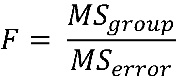
| Between treatments | k – 1 | SST | MST | MST/MSE |
| Error | N – k | SSE | MSE |
N = total number of observations for the entire experiment = n(k)
k = Number of treatments or groups
The F-statistic is always presented along with the df values,
e.g. F(MST, MSE) = F-ratio, p-value
- ANOVA conducted on a one-factor design is called a one-way ANOVA.
- That on a two-factor design is a two-way ANOVA.
Test based on two estimates of the population variance:
- Mean square error (MSE): computed from sample variances.
- Mean square treatment (MST): computed from the sample means.
MSB is larger than MSE when the population means are not equal. Comparing MSE and MSB is a critical step in ANOVA. Finding a larger MSB than MSE is a sign that the population means are not equal. The probability of getting MSB that large or larger if the population means were all equal is based on the F-ratio (ratio of MST to MSE) i.e. a ratio between the differences in the means of the groups and the error variance.
- So the differences among the means are thought of as their variance.
- Higher variance among the means indicates that there are more differences.
- The variance among the group means is called the between-groups variance.

A larger ratio indicates that the differences between the groups are greater than the error or “noise” going on inside the groups. If this ratio, the F-statistic, is large enough given the size of the sample, we can reject the null hypothesis. The sample size will affect the outcome because large samples allow for better tests of the null hypothesis.
Tests the hypothesis of no difference (null hypothesis), when the null hypothesis is rejected, the conclusion is that at least one population mean is different from at least one other mean.
- ANOVA used to study the effect of k (>2) levels of a single factor.
- To determine if different levels of the factor affect measured observations differently, the following hypotheses are tested.
H0: mi = m all i = 1, 2, . . ., k
H1: mi = m some i = 1, 2, . . ., k
- Where mi is the population mean for level i.
Example
Suppose that one is investigating the effect of four different temperatures (100, 150, 200, 250oC) on the response variable (loaf volume) of bread.
- Samples from each treatment were obtained and analyzed for loaf volume.
- The first step in the analysis is to write the statistical model for each observation as follows:
- The loaf volumes in the experiment may be different and we may be tempted to conclude that the differences exist due to the baking temperatures.
- However, this difference may also be the result of certain other factors which are attributed to chance and which are beyond human control- a factor termed “error”
- Thus, estimates of the amount of variation due to assignable causes (or variance between samples) as well as due to chance (or variance within the samples) are obtained separately and compared using the F-test and conclusions are drawn using the value of F.
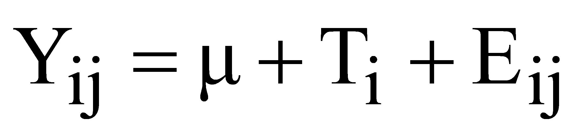
i = 1, 2, …, n
j = 1, 2, …, k
Yij = the observed loaf volume for the ith treatment and jth observation,
- = the grand mean for all observations,
Ti = the effect of the ith treatment and
Eij = random errors.
ANOVA Assumptions
- Assumption #1: Dependent variable should be measured at the interval or ratio scale
- Assumption #2: The Independent variable should consist of three or more categorical, independent groups. For just two groups and an independent-sample t-test is commonly used.
- Assumption #3: The observations should be independent- i.e. there is no relationship between the observations in each group or between the groups themselves.
- Assumption #4: There should be no significant outliers.
- Assumption #5: The dependent variable should be approximately normally distributed for each category of the independent variable. Requires approximately normal distribution because one-way ANOVA is quite “robust” to violations of normality, meaning that assumption can be a little violated and still provide valid results. The normality assumption tested with the Shapiro-Wilk test of normality.
- Assumption #6: There needs to be a homogeneity of variances. Tested using Levene’s test for homogeneity of variances. May run Welch ANOVA if data fails assumption.